Introduction to Deep Learning with PyTorch

Quentin Wach

(Note, June 14, 2025.) This blog post was originally drafted many years ago. Changes were made to the code, some of the writing, and the graphics are reworked entirely.

This has been done a thousand times before by many others before me. But the learning happens as it is done. So let’s repeat it once more for the sake of growth.

Introduction

PyTorch is an open-source deep learning framework developed by Facebook’s AI Research lab (FAIR) and released in 2016. The name stands out for its dynamic computation graph. This means that every time you execute a forward pass, PyTorch constructs the graph on-the-fly, based on the actual operations and control flow (loops, conditionals, etc.) in your Python code, whereas TensorFlow (at least before 2.0) fixed its graph before execution. Before PyTorch, the deep learning landscape was shaped by several influential libraries, but let’s crack on!

In this blog post, we’ll explore the core ideas behind deep learning frameworks like PyTorch. We’ll start by revisiting the basics of neural networks with a simple Perceptron and then break down backpropagation, computational graphs, automatic differentiation, the training loop and provide a sumoke example in PyTorch. (We will skip explanations of JIT here though.)

The Good Old Perceptron

I did this the first time when I was 16 and actually repeated it quite often back then as I was just learning to program. Let me recall it yet another time as a foundation for what’s to come.

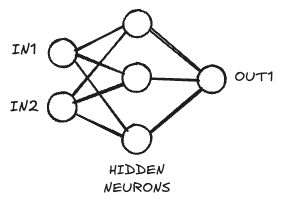
Let’s say we want to train a neural network to model a simple logic gate like an NAND gate. It has two binary inputs and one output, so our network should be structured the same. We’ll add three hidden neurons in-between, and our neurons will all have simple sigmoid activation functions with signals compressed between 0 and 1.

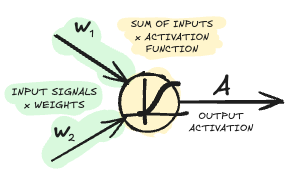
This is a dense neural network, so all neurons in the input layer \(L_1\) are connected to all the neurons in the hidden layer \(L_2\) and so on. For every single neuron, we sum up all the input signals multiplied by the weights of the connections to that neuron, feed it through a non-linear activation function, and return the output. Easy.

Forward Pass

Now, instead of using a for-loop over all the nodes and edges, we can actually express the computation of the entire network with some matrix algebra. First, we compute the input to the node, which is a simple matrix transformation of the input signals with the weights to get the inputs to the hidden neurons.

Here’s how we can implement this simple network in PyTorch:

import torch
import torch.nn as nn

# Define a simple neural network
class SimpleNet(nn.Module):
    def __init__(self):
        super().__init__()
        self.layer1 = nn.Linear(2, 3)  # 2 inputs -> 3 hidden
        self.layer2 = nn.Linear(3, 1)  # 3 hidden -> 1 output
        self.sigmoid = nn.Sigmoid()
    
    def forward(self, x):
        x = self.sigmoid(self.layer1(x))
        x = self.sigmoid(self.layer2(x))
        return x

# Create model and input
model = SimpleNet()
inputs = torch.tensor([[0., 0.]])  # Example input
output = model(inputs)

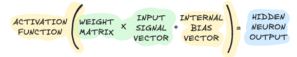
We then compute the activations for all the nodes in the layer (including a bias offset \(\vec{b}_k\)), in general

\[\vec{L}_{k}^{out} = f_k(\textbf{W}_{k} \cdot \vec{L}_{k-1}^{out} + \vec{b}_{k})\]

where, here, \(f_k\) is the activation function

\[f_k(x) = \frac{1}{1 + e^{-x}}\]

and \(\textbf{W}_{k}\) is the matrix of weights that maps the outputs of layer \(k-1\) to the inputs of layer \(k\), and \(\vec{b}_{k}\) is the bias vector for the hidden layer. We simply repeat this for every following layer (if we had any here) until all neurons “fired”.

QUESTION: Why do we have custom weights for every connection but the same activation function for all the nodes within a layer? - ANSWER: Practical reasons. To inject consistent non-linearity which we can more easily interpret and, importantly, to maintain computational efficiency. Though there is research exploring ideas that vary the activation within the layer e.g. “Kolmogorov–Arnold Networks”¹.

Error Backpropagation and Computational Graphs

Brace yourself. Math coming up.

When training a neural network, our goal is to minimize the difference between the network’s predictions and the true targets. This difference is quantified by a loss function, such as mean squared error for regression or cross-entropy for classification.

To optimize the network, we need to compute how each parameter (weight and bias) contributes to the loss, and then adjust them to reduce the error. This is where backpropagation comes in.

Backpropagation is an efficient algorithm for computing gradients of the loss with respect to all parameters in the network by applying the chain rule of calculus through the layers. When we consider a simple feedforward network as shown in the previous section, the final output \(\hat{y}\) is compared to the target \(y\) using a loss function \(\mathcal{L}(\hat{y}, y)\).

To update the parameters, we need the gradients \(\frac{\partial \mathcal{L}}{\partial \textbf{W}_k}\) and \(\frac{\partial \mathcal{L}}{\partial \vec{b}_k}\) for each layer \(k\). Using the chain rule, we propagate the gradient of the loss backward through the network

\[\frac{\partial \mathcal{L}}{\partial \textbf{W}_k} = \frac{\partial \mathcal{L}}{\partial \vec{L}_k^{out}} \cdot \frac{\partial \vec{L}_k^{out}}{\partial \textbf{W}_k}\]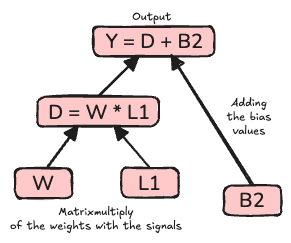

and similarly for the biases. The key insight is that the gradient at each layer depends on the gradient from the layer above, multiplied by the local derivative at the current layer. This recursive application of the chain rule is what makes backpropagation efficient.

To keep track of all these dependencies, we represent the computation as a directed acyclic graph (DAG)², called the computational graph³⁴. Each node in the graph is an operation (like matrix multiplication, addition, or activation), and the edges represent the flow of data. During the forward pass, we compute the outputs and remember how each value was computed.

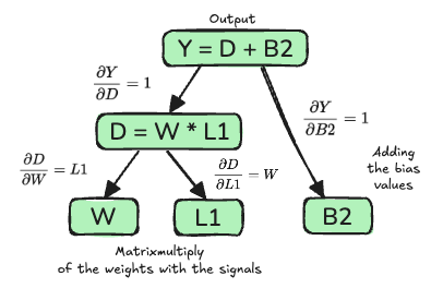
During the backward pass, we traverse the graph in reverse, applying the chain rule at each node to accumulate gradients.

\[\begin{align*} \frac{\partial Y}{\partial D} \cdot \frac{\partial D}{\partial L1} &= W \\ \frac{\partial Y}{\partial D} \cdot \frac{\partial D}{\partial W} &= L1 \\ \frac{\partial Y}{\partial B2} &= 1 \\ \end{align*}\]

Note that the graph shown here is an oversimplification as, in reality, the DAG branches off into every single mathematical operation which quickly becomes very complex since, for example, matrix multiplication contains many individual multiplication and addition operations.

But that is exactly why such a computational graph has its perks. It lets users build and manipulate models at a high level while it automatically handles chaining of operations and gradients, and enables visualization, debugging, and introspection.

Here’s how PyTorch handles the computational graph and backpropagation:

# Enable gradient tracking
x = torch.tensor([[0., 0.]], requires_grad=True)
model = SimpleNet()

# Forward pass
output = model(x)

# Compute loss
target = torch.tensor([[1.]])
loss = nn.MSELoss()(output, target)

# Backward pass - PyTorch automatically builds and traverses the computational graph
loss.backward()

# Now gradients are available
for name, param in model.named_parameters():
    print(f"{name} gradient:", param.grad)

Optimization

Once all gradients are computed, the parameters are updated using an optimization algorithm such as ADAM or stochastic gradient descent (SGD)

\[\theta \leftarrow \theta - \eta \frac{\partial \mathcal{L}}{\partial \theta}\]

where \(\theta\) represents a parameter (weight or bias) and \(\eta\) is the learning rate.

We start with random values for the model’s parameters (the weights and biases). For a randomly selected data point (or a small batch) we then compute the gradient of the loss function with respect to each parameter as explained before. We then adjust each parameter in the opposite direction of the gradient by a small step (the learning rate). This process is repeated for many iterations, gradually improving the network’s performance as we descent the gradient of the optimization space.

NAND Logic Gate Example

Let’s train the neural network to learn to act like a NAND logic gate. Here is the complete code to do so:

import torch
import torch.nn as nn
import numpy as np

# Define a simple neural network
class SimpleNet(nn.Module):
    def __init__(self):
        super().__init__()
        self.layer1 = nn.Linear(2, 3)  # 2 inputs -> 3 hidden
        self.layer2 = nn.Linear(3, 1)  # 3 hidden -> 1 output
        self.sigmoid = nn.Sigmoid()
    
    def forward(self, x):
        x = self.sigmoid(self.layer1(x))
        x = self.sigmoid(self.layer2(x))
        return x

# NAND gate training data
# NAND truth table: [0,0]->1, [0,1]->1, [1,0]->1, [1,1]->0
inputs = torch.tensor([[0., 0.], [0., 1.], [1., 0.], [1., 1.]])
targets = torch.tensor([[1.], [1.], [1.], [0.]])

# Create model and optimizer
model = SimpleNet()
optimizer = torch.optim.SGD(model.parameters(), lr=0.5)
criterion = nn.MSELoss()

# Track training progress
losses = []
epochs = 4000

# Training loop
for epoch in range(epochs):
    # Forward pass
    outputs = model(inputs)
    loss = criterion(outputs, targets)
    
    # Backward pass
    optimizer.zero_grad()
    loss.backward()
    optimizer.step()
    
    # Track loss
    losses.append(loss.item())

It is a dense neural network as shown initially in this post with two input neurons, three hidden neurons and a single output neuron trained using SGD with an initial learning rate of 0.5 over 4000 iterations. We are tracking the losses in a list.

The results are visualized with an additional script using Matplotlib and are shown in the figure below:

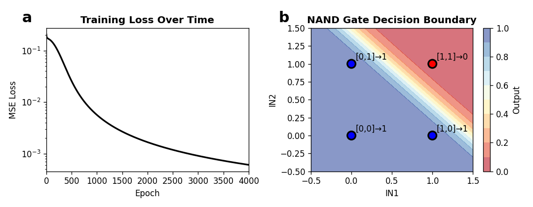
The MSE loss declines nicely and our predictions are close to what we wanted.