Vector-Quantized Variational Autoencoders

Quentin Wach

Introduction

This is a minimal implementation of a vector-quantized variational autoencoder to encode and decode the MNIST dataset. I recommend you also read the original papers by Aaron van den Oord et al. (2018)¹ and Ali Razavi et al. (2019)².

What Are Autoencoders?

In machine learning, we often want to compress high-dimensional data (like images) into a lower-dimensional representation that still captures the essential information. This is useful for tasks like denoising, generative modeling, and unsupervised learning. Autoencoders (AEs) are neural networks trained to encode data into a compact latent space and then decode it back to reconstruct the original input. However, standard AEs learn a deterministic mapping and do not provide a meaningful structure to the latent space, making them less useful for generative tasks.

Variational Autoencoders (VAEs)³⁴ address this by introducing a probabilistic framework: they learn to encode inputs as distributions (typically Gaussian) in the latent space rather than encoding to a single point in that space, enabling smooth interpolation and sampling by mapping each point from a large complex dataset into a distribution within the latent space. VAEs are powerful generative models, but their reliance on continuous latent variables can be limiting when the underlying data has inherently discrete structure (e.g., language, symbolic data, or even certain image features).

Why Vector-Quantization?

This is what VQ-VAEs are attempting to resolve. They introduce a discrete latent space by quantizing the encoder output using a learned codebook of embeddings. This allows the model to represent data using a finite set of vectors, which can be more interpretable and better suited for tasks like compression, clustering, and symbolic reasoning. VQ-VAEs have also been shown to improve generative modeling in domains like images, audio, and language.

Implementation

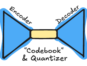
Let’s work through how to build one. VQ-VAE consists of an encoder, an embedding (or a “codebook”) and a decoder. When an image is passed as input, it is converted into latent vectors using the encoder network. The embedding space consists of many latent vectors, which are compared to that of the input one. The distances are calculated and the most similar (least distance) latent vector (in the embedding space) to the input’s latent vector is selected. The selected one is then fed into the decoder network which reconstructs the image.

Here is my attempt at a detailed overview:

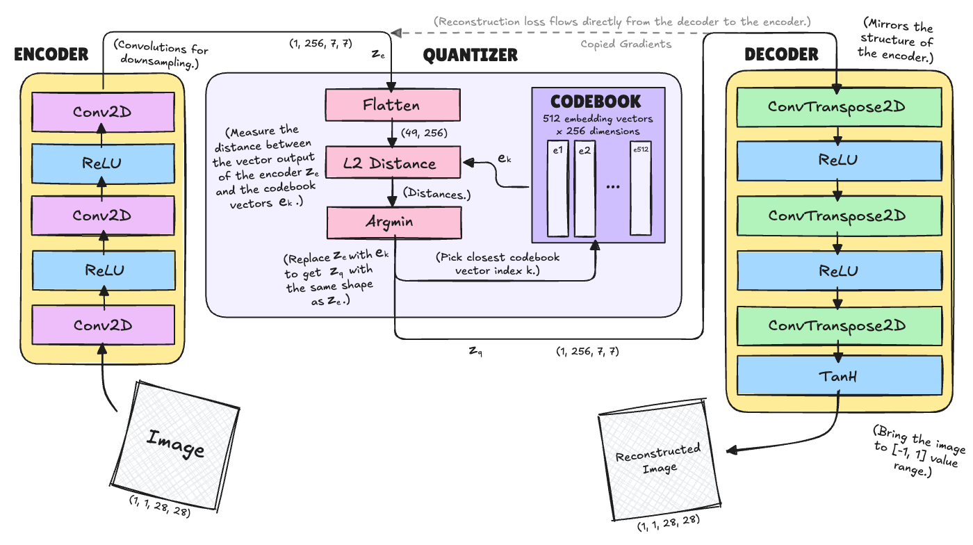
Importantly, we can’t just backpropagate the error gradient through this naively. Instead, we have to stop the gradients and update the codebook more manually whith the encoder being updated directly from the signal of the decoder.

But let’s go through this from left to right.

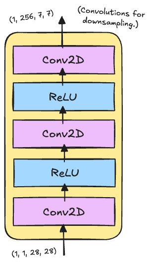
Encoder

The encoder is responsible for transforming the input images into a compressed latent representation that captures the essential features needed for reconstruction. In our VQ-VAE implementation, the encoder uses a simple convolutional architecture designed specifically for MNIST’s characteristics.

Starting with 28×28 grayscale images, it applies two strided convolutions to reduce spatial resolution to 7×7, followed by a final convolution that maps to the embedding dimension. The use of ReLU activations after the first two layers introduces non-linearity while the final layer has no activation to allow the vector quantizer to work with unbounded values.

class Encoder(nn.Module):
    def __init__(self, input_channels=1, hidden_dim=64, output_dim=256):
        super(Encoder, self).__init__()
        self.conv1 = nn.Conv2d(input_channels, hidden_dim, kernel_size=4, stride=2, padding=1)
        self.conv2 = nn.Conv2d(hidden_dim, hidden_dim, kernel_size=4, stride=2, padding=1)
        self.conv3 = nn.Conv2d(hidden_dim, output_dim, kernel_size=3, stride=1, padding=1)
        
    def forward(self, x):
        x = F.relu(self.conv1(x))
        x = F.relu(self.conv2(x))
        x = self.conv3(x)
        return x

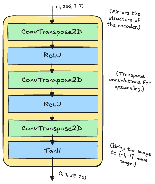
Decoder

The decoder performs the inverse operation of the encoder, transforming the (quantized) latent representations back into reconstructed images. It mirrors the encoder’s architecture but uses transposed convolutions.

Note that, unlike regular convolutions that reduce spatial dimensions, transposed convolutions increase them by learning an upsampling operation. They work by inserting zeros between input elements and then applying a convolution, effectively “stretching” the feature maps. (For example, a transposed convolution with stride=2 doubles the spatial dimensions, allowing us to go from 7×7 back to 28×28 through two upsampling steps.)

The tanh activation on the final layer ensures outputs are bounded between [-1, 1], appropriate for normalized image data.

class Decoder(nn.Module):
    def __init__(self, input_dim=256, hidden_dim=64, output_channels=1):
        super(Decoder, self).__init__()
        self.conv1 = nn.ConvTranspose2d(input_dim, hidden_dim, kernel_size=3, stride=1, padding=1)
        self.conv2 = nn.ConvTranspose2d(hidden_dim, hidden_dim, kernel_size=4, stride=2, padding=1)
        self.conv3 = nn.ConvTranspose2d(hidden_dim, output_channels, kernel_size=4, stride=2, padding=1)
        
    def forward(self, x):
        x = F.relu(self.conv1(x))
        x = F.relu(self.conv2(x))
        x = torch.tanh(self.conv3(x))
        return x

Quantizer & Codebook

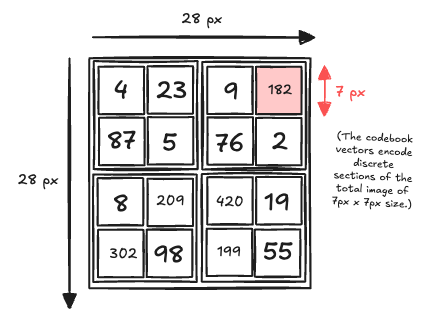
In the design shown above, the images are split into 7×7 pixel patches each of which we need to design a code vector to. Now, this is the tricky part that requires some thinking:

The vector quantizer discretizes the encoder’s continuous outputs by mapping each latent vector to its nearest entry in a learnable codebook of \(k\) embeddings. This process enables the model to represent data using a finite set of prototypes, forming the discrete bottleneck at the heart of VQ-VAE.

Step-by-step:

Compute the L2 distance between each \(z_e\) vector and each codebook embedding \(e_k\).
For each location, pick the nearest codebook entry’s index \(k^*\) using argmin.
Replace \(z_e\) at that location with \(e_{k^*}\) to get \(z_q\) (same shape as \(z_e\) but values are discrete embeddings).

The decoder then learns to reconstructs the image from \(z_q\) rather than \(z_e\).

Because the nearest neighbor step is non-differentiable, a straight-through estimator is used: gradients are copied from the quantized output \(z_q\) back to the encoder output \(z_e\), allowing end-to-end training despite the discrete step.

But we also need to update the codebook! How do we do that?

Losses

We need to calculate a codebook losst and commitment loss in addition to the reconstruction loss (mentioned before). So we have three terms:

\[\mathcal{L} = \underbrace{\| x - \hat{x} \|^2}_{\text{reconstruction loss}} + \underbrace{\| \text{sg}[z_e] - e \|^2}_{\text{codebook loss}} + \beta \underbrace{\| z_e - \text{sg}[e] \|^2}_{\text{commitment loss}}\]

where sg[·] means “stop gradient” (no gradient flows through this variable in this term).

The codebook loss updates the embedding vectors \(e\) to be closer to the encoder output \(z_e\) (encoder is stopped here). The commitment loss updates the encoder to produce outputs closer to the selected codebook vector \(e_{k^*}\) (codebook is stopped here). And the reconstruction loss gradients flow from the decoder output back to \(z_q\) and are copied to \(z_e\) (straight-through estimator).

I’ll repeat this in more detail since this is important:

1. Reconstruction Loss

This is the primary loss that measures how well the model can reconstruct the input images. It optimizes both the encoder and decoder to minimize the difference between the original input \(x\) and the reconstructed output \(\hat{x}\):

\[\mathcal{L}_{recon} = \mathbb{E}_{x \sim p(x)} \left[ \|x - \hat{x}\|^2 \right]\]

This is implemented as Mean Squared Error (MSE) between the input and reconstructed images.

2. Codebook Loss

Since the quantization step is non-differentiable, gradients cannot flow directly through the codebook lookup. The codebook loss ensures that the codebook vectors \(e_k\) move towards the encoder outputs \(z_e\):

\[\mathcal{L}_{codebook} = \|\text{sg}[z_e(x)] - e\|^2\]

This loss only updates the codebook vectors, pulling them closer to the encoder representations. But there is an issue we need to correct still with our final loss…

3. Commitment Loss

Without the commitment loss, the encoder could produce outputs that grow arbitrarily far from the codebook vectors, making quantization ineffective. The commitment loss ensures the encoder “commits” to producing outputs close to the codebook:

\[\mathcal{L}_{commit} = \beta \|z_e(x) - \text{sg}[e]\|^2\]

where \(\beta\) is a hyperparameter (typically 0.25) that controls the weight of the commitment loss relative to other components.

Below the code that implements all of this:

class VectorQuantizer(nn.Module):
    def __init__(self, num_embeddings=512, embedding_dim=256, commitment_cost=0.25):
        super(VectorQuantizer, self).__init__()
        
        self.embedding_dim = embedding_dim
        self.num_embeddings = num_embeddings
        self.commitment_cost = commitment_cost
        
        # Initialize codebook with random vectors
        self.embedding = nn.Embedding(num_embeddings, embedding_dim)
        self.embedding.weight.data.uniform_(-1/num_embeddings, 1/num_embeddings)
        
    def forward(self, inputs):
        # Flatten input to [batch_size * height * width, embedding_dim]
        flat_input = inputs.view(-1, self.embedding_dim)
        
        # Calculate L2 distances between input and codebook vectors
        distances = (torch.sum(flat_input**2, dim=1, keepdim=True) 
                    + torch.sum(self.embedding.weight**2, dim=1)
                    - 2 * torch.matmul(flat_input, self.embedding.weight.t()))
        
        # Find closest codebook vectors
        encoding_indices = torch.argmin(distances, dim=1).unsqueeze(1)
        
        # Get quantized vectors
        quantized = self.embedding(encoding_indices).view(inputs.shape)
        
        # Calculate VQ loss
        e_latent_loss = F.mse_loss(quantized.detach(), inputs)  # Commitment loss
        q_latent_loss = F.mse_loss(quantized, inputs.detach())  # Codebook loss
        loss = q_latent_loss + self.commitment_cost * e_latent_loss
        
        # Straight-through estimator: copy gradients from quantized to input
        quantized = inputs + (quantized - inputs).detach()
        
        return quantized, loss, encoding_indices


class VQVAE(nn.Module):
    def __init__(self, num_embeddings=30, embedding_dim=256, commitment_cost=0.25):
        super(VQVAE, self).__init__()
        
        self.encoder = Encoder(output_dim=embedding_dim)
        self.vq = VectorQuantizer(num_embeddings, embedding_dim, commitment_cost)
        self.decoder = Decoder(input_dim=embedding_dim)
        
    def forward(self, x):
        # Encode
        z_e = self.encoder(x)
        
        # Quantize
        z_q, vq_loss, encoding_indices = self.vq(z_e)
        
        # Decode
        x_recon = self.decoder(z_q)
        
        return x_recon, vq_loss, encoding_indices

# Initialize model
model = VQVAE().to(device)
optimizer = optim.Adam(model.parameters(), lr=1e-3)

Training

The training process for VQ-VAE involves optimizing both the reconstruction quality and the discrete codebook learning simultaneously. I chose a batch size of 64. The Adam optimizer with a learning rate of 1e-3 provides stable convergence. Here is the concrete implementation. Standard stuff.

# Training function
def train_epoch(model, train_loader, optimizer, device):
    model.train()
    total_loss = 0
    total_recon_loss = 0
    total_vq_loss = 0
    
    for batch_idx, (data, _) in enumerate(train_loader):
        data = data.to(device)
        optimizer.zero_grad()
        
        # Forward pass
        recon_data, vq_loss, _ = model(data)
        
        # Calculate losses
        recon_loss = F.mse_loss(recon_data, data)
        total_loss_batch = recon_loss + vq_loss
        
        # Backward pass
        total_loss_batch.backward()
        optimizer.step()
        
        total_loss += total_loss_batch.item()
        total_recon_loss += recon_loss.item()
        total_vq_loss += vq_loss.item()
        
        if batch_idx % 200 == 0:
            print(f'Batch {batch_idx}, Loss: {total_loss_batch.item():.4f}, '
                  f'Recon: {recon_loss.item():.4f}, VQ: {vq_loss.item():.4f}')
    
    return (total_loss / len(train_loader), 
            total_recon_loss / len(train_loader), 
            total_vq_loss / len(train_loader))

# Training loop
num_epochs = 5  # Minimal training for demonstration
losses = []

print("Starting training...")
for epoch in range(num_epochs):
    avg_loss, avg_recon, avg_vq = train_epoch(model, train_loader, optimizer, device)
    losses.append(avg_loss)

# Plot training loss
plt.figure(figsize=(10, 4))
plt.subplot(1, 2, 1)
plt.plot(losses)
plt.title('Training Loss')
plt.xlabel('Epoch')
plt.ylabel('Loss')
plt.grid(True)

Results & Conclusion

The reconstructions show that the model captures the essential features of handwritten digits, including stroke patterns and digit shapes, despite the significant compression and discretization.

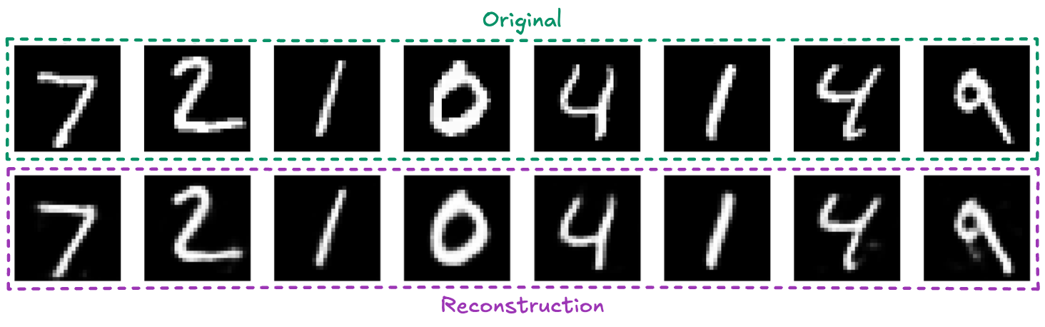
That is for the case of a codebook with 40 entries.

Codebook Size and Impact

The size of the codebook is a crucial hyperparameter. A small codebook forces the model to reuse codes, which can lead to more generalization but may limit expressiveness and reconstruction quality if too small. A large codebook increases the capacity to represent diverse features, but can lead to underutilization (many codes never used) and may require more data to train effectively.

In this case, with a codebook of 40 entries, all codes were used (100% utilization), indicating efficient use of the discrete space. With a larger codebook of 512 entries, only about 54% were used, suggesting redundancy but also more capacity for complex data. And for 20 entries, only 12 were used, all images collapsed to black, i.e. the network failed entirely to encode the MNIST dataset.

Compression

I also want to just hint at the importance of the design of the VAE architecture, importantly, the compression! There are a lot of VAEs floating around on the web but they all perform differently. At the same time, many using diffusion models to generate images often wonder why there are these weird arifacts especially in the details. This article⁵ states it well:

“For SDXL VAE, where C=4: 3×64/4=48 For FLUX VAE, where C=16: 3×64/16=12

Therefore, SDXL VAE compresses images 48 times smaller, while FLUX VAE compresses only 12 times smaller, preserving more details. This difference is significant: SDXL VAE compresses images 4 times more aggressively than FLUX VAE, which explains why FLUX preserves substantially more fine details in the generation process.”

Future

We may discuss the problem of codebook collapse in the future.

But more importantly, we want to generate new images using our VQ-VAE! To do so, we need to learn how to use the codebook indices to construct new images. This can be done auto-regressively using a Language Transformer, using a Diffusion Model, or a GAN. There is a lot to be said and to be explored here which is quite interesting in the research literature. Notably, creating images in latent space leads to much higher quality images while also being much more efficient than diffusion in pixel space which is one of the major ideas Stable Diffusion and future models have been builing on.