Dubins Paths for Waveguide Routing

(Updated: March 12, 2024.) I deleted the majority of the code I presented when I posted this first as it was quite hacky and all the recources can be found in the links below. It should also be added that, while much of the photonics community does not seem to be aware of Dubins paths and instead talk about s-bends and so on, I believe libraries already implement similar methods and Dubins paths are more or less just a generalization that can make life easier at times. It sure did for me and my work.

What does the perfect waveguide routing look like? Traditional waveguide interconnects lack efficiency and optimization, leading to suboptimal photonic integrated circuits (PICs). Addressing key concerns like minimizing internal and radiation losses, reducing cross-talk, and avoiding unnecessary crossings, I explored the concept of finding the shortest path between two points in a PIC given a minimum bending radius. Dubins paths, already well known in robotics and control theory, emerged as a simple and highly practical solution.

1 Introduction

I’ll try to keep this short and not ramble too much. I just want to get this out there since I found it rather useful and can’t believe it isn’t yet standard.

When I started my work on layouts for photonic integrated circuit in September 2023, it became quickly obvious that the typical waveguide interconnects provided by libraries are not well behaved nor optimal as to improve the performance and compactness of the photonic integrated circuit. Most commonly, we have simple straights, circular arcs, all sorts of splines, as well as Euler-bends, in short: They are all simple analytical functions or splines that (try to) optimize themselves. All of these are either simple building blocks that leave most of the work to the designer who has to plan out and specify every route, or behave extremely poorly and lead to overly bendy results that may even cross each other.

So in my first two weeks there, I was thinking about what we have to consider. Waveguides have to fullfil multiple criteria. They need to be…

As short as possible as to minimize internal losses.
As straight and continuos as possible as to minimize radiation losses.
As far away from other waveguides and structures as to minimize cross-talk.
Does not cross other waveguides unless close to a 90° angle if absolutely necessary.

It became quickly obvious that trying to find an optimum for all these design parameters is impossible unless we either weigh their importance using a complicated metric we have to justify, or make much harder constraints. Since it is common to have a fixed minimum bending radius for waveguides, it makes sense to translate this here. I then boiled all of the considerations down to the single, I believe, most important question: “What is the shortest path between the pin or vector \(\vec{a}\) and pin or vector \(\vec{b}\) given a minimum bending radius?”

As it turns out, the answer is rather simple and long established in the field of robotics / control theory. Dubins paths!

2 What are they?

Dubins paths are named after Lester Dubins, who introduced them in the 1950s¹. They refer to the shortest paths that a vehicle can take from one point to another while constrained to move at a specific minimum turning radius. These paths are thus commonly studied in the field of motion planning for vehicles, particularly in robotics and aerospace engineering.

dubin1

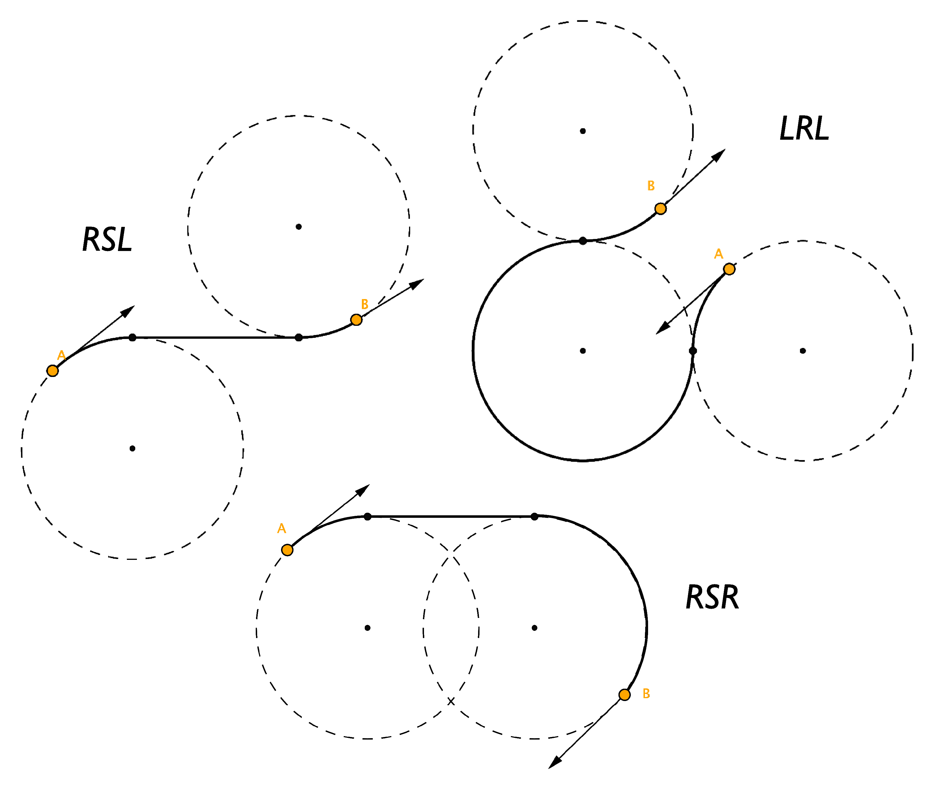
These paths simply connect circular arcs with straights which leaves us with a couple of characteristic Dubins paths:

LRL (Left-Right-Left)
RLR (Right-Left-Right)
LSL (Left-Straight-Left)
RSR (Right-Straight-Right)
LSR (Left-Straight-Right)
RSL (Right-Straight-Left)

You can see three examples of the possible paths in the figure I adapted here².

3 Geometric Construction

Dubins did indeed prove that these trajectories are the shortest paths mathematically. The geometric construction is quite intuitive and a nice toy problem to figure out on ones own but it can quickly explode into multiple pages of pen and paper calculations and diagrams which is why I am not going to go into it here. Instead, I refer to a great overview and explanation of the synthesis of Dubins paths given by David A. Anisi³. A wonderful and in-depth guide is also given by Andy G⁴.

4 Code

There is an abundance of implementations of Dubins paths available on the internet⁵.

It doesn’t take much time to either do an implementation from scratch or adapt preexisting code. We can then wrap it all up into a single, simple to use function just like any other provided by the design library you might be using. In this case, I have been using the Nazca library⁶ which comes with several interconnects, including straights and circular arcs which are used often but very tedious and slow to work with alone. Using dubin_p2p(), we can simply define the start pin, the end pin, and our code will route a Dubins path between them using the straights and circular arcs provided by Nazca. Of course, this can be easily adapted to other tools like GDSFactory⁷.

#########################################################################
# Use this when designing your PIC with Nazca!
#########################################################################

# Create Dubins path between two pins in Nazca
def dubin_p2p(xs, pin1, pin2, radius=500, width=4):
    """
    Finds and creates the shortest possible path between two vectors
    (pin1 and pin2) with a minimum bending radius,
    a so called "Dubins path". This Dubins path is made of two
    circular bends and a straight waveguide.
    Returns a cell containing these waveguides.

    IMPORTANT
    =========
    In this version, you NEED to specify to put the path at the starting
    pin so if pin1=IO.pin["a0"] you must add .put(IO.pin["a0"]).
    Else, the Dubins path will be generated correctly
    but possibly at the wrong position. 
    
    PARAMETERS
    ==========
    xs:     Crosssection parameters.
    pin1:   The start pin to which the Dubins path attaches.
    pin2:   The end pin to where the Dubins path ends.
    radius: The minimum bending radius for the Dubins paths.
    width:  The width of the waveguides dubin_p2p creates.
    """
    # Get the pin vectors from pin1 and pin2
    START = pin1.xya()
    END = pin2.xya()

    # Change the angle for the second pin
    new_end = list(END)
    new_end[2] = new_end[2] - 180
    END = tuple(new_end)

    # Find the Dubins path between pin1 and pin2
    path = dubins_path(start=START, end=END, radius=radius)

    # Create the Dubins path with nazca using bends and straights
    return gds_solution(xs, pin1, pin2, solution=path)

5 Conclusion

In the figure below, a comparison between a dense array of Dubins paths and arrays using Nazcas s-bends and cobra splines is made:

sleep_figure_1

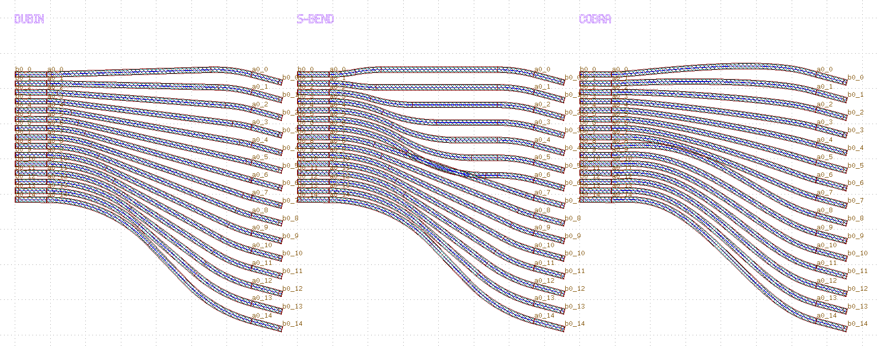
As one can see, not only do other interconnects lead to over-bending of the waveguides and thus a longer path and greater losses, they are also less reliable, predictable, often break the design rules to not violate the minimum bending radius as is indeed the case here. They even intersect each other! Meanwhile, the Dubins paths behave extremely predictably. They clearly show the shortest path without unnecessary bends and they do not intersect each other which allows for much denser layouts than would be possible with the other interconnects. What I realized only after this was that there are indeed interconnects provided by Nazca which are essentially Dubins paths like bend_strt_bend_p2p() though not as general.

Also, there is a list of improvements one may make based on this. For one, the curvature of Dubins paths are not smooth which may lead to higher radiation losses. The hours of headaches I personally avoided just by using Dubins paths are insane. It is also simply much more enjoyable to use.

That’s my little tip for those working on photonic integrated circuit layouts. I hope it helps!

1 Introduction

2 What are they?

3 Geometric Construction

4 Code

5 Conclusion

References